abstract
This post presents a method to identify the order of linear multidimensional (nD) systems based on rank conditions of a recursive hankel matrix. A recursive hankel matrix is a generalization of a classical hankel matrix for multidimensional systems. The estimation method is based on the intersection algorithm for one-dimensional systems. At the basis of this algorithm lies the intersection between past and future data. This subspace contains the information of the sate sequence. This post extends the concept of past and future data to nD systems and introduces the concept of mode\(-k\) left and right data. The intersection between two mode\(-k\) left and right matrices reveals the order of the system in dimension \(k\). The result of this post is a method to estimate the order of a partial difference equation from observed input-output data.
This post is inspired my the work published in Order estimation of two dimensional systems based on rank decisions [1]. The full list of authors of this paper are
- Bob Vergauwen
- Oscar Mauricio Agudelo
- Bart De Moor
Introduction
In recent years increasing attention in system theory is paid to multidimensional dynamical systems, so-called nD systems [2]. nD systems are systems characterized by signals that depend on several independent variables. These variables are, for example, space and time. Important model classes for such systems are partial differential equations (PDE’s) and partial difference equations (PdE’s), for which the ‘order’ can be different in each independent variable. For example, the parabolic heat equation is of second order in space and first order in time.
In this post the ideas of the intersection algorithm [3] for subspace identification are explored and partially extended to two dimensional systems. The notion of the recursive Hankel matrices (\(H_{r}\)) is introduced [4]. The left-null space of this matrix contains the information of the coefficients of the PdE. By calculating the dimensions of the linear intersection between two recursive Hankel matrices, it is possible to estimate the order of the linear dynamical system.
The presented algorithm is summarized as follows.
- Hankelize the observed output (and possibly input) data.
- Divide the Hankel matrices in Left, Right, Top and Bottom Hankel matrices.
- Calculate the dimension of the linear intersection between the matrices.
- Based on the dimension of the intersection, the order of the PdE is calculated.
The outline of this post is as follows. In Section the two-dimensional representation of a linear system is presented as well as the concept of a stencil, which is a graphical tool used to represent linear multidimensional systems. In Section the main tool of our algorithm is defined, namely the recursive Hankel matrix. This is a direct extension of a Hankel matrix to multidimensional datasets. In Section the rank of a recursive Hankel matrix is discussed. Two propositions are provided relating the rank of the recursive Hankel matrix to the order of a PdE. In Section the concept of past and future Hankel matrices is extended to left, right top and bottom matrices. In Section it is shown that the intersections between respectively the left and right, top and bottom Hankel matrices reveal the order of a 2D system. To illustrate all concepts, Section presents an example where simulated data of the transport-diffusion equation is used to estimate the order of the underlying equations. Finally, in Section the conclusions are formulated.
Multidimensional systems
Multidimensional systems are systems that depend on several independent variables, for example, space and time. Although several state space models have been proposed (Givone and Roesser [5], Attasi [6] and Kurek [7] to represent linear nD systems, in this post we will work with PdEs that describe their dynamics.
A linear two-dimensional input-output discrete system can be represented by the following difference equation,
\begin{multline} \label{eqn:nDsystemDiscrete} \sum_{i=0}^{n_{1}} \sum_{j=0}^{n_{2}} \alpha_{i,j}y[k_{1}+i,k_{2}+j] = \\ \sum_{i=0}^{o_{1}} \sum_{j=0}^{o_{2}} \beta_{i,j}u[k_{1}+i,k_{2}+j], \end{multline}
where input and output of the system are respectively denoted by \(u[k_{1},k_{2}]\) and \(y[k_{1},k_{2}]\). The values \(k_{1}\) and \(k_{2}\) are two discrete shift variables. The order of the output dynamics is defined as the tuple \((n_{1},n_{2})\), the order of the input dynamics is \((o_{1},o_{2})\). The order of the system is defined as the tuple,
\begin{equation} O_{s} = (\text{max}(n_{1},o_{1}),\text{max}(n_{2},o_{2})). \end{equation}
This order definition indicates how many neighboring data points are linearly related.
Stencil representation
A common method for representing discrete nD systems in a graphical way is by using stencils [8]. A stencil is a geometrical tool that illustrates the linear relations between adjacent grid points in a multidimensional dataset. As an example the Crank-Nicolson stencil is shown in Figure 1 this stencil is often used in the simulation of the 1D heat equation. The gray and black points represent data points. The black lines connecting the points represents linear relations between six adjacent data points. In the field of numerical simulation of partial differential equations, the black point is calculated from the available data in the gray points. The difference equation associated to this stensil is equal to,
\begin{multline*}\label{key} y[k_{1}+1,k_{2}+1] = \alpha_{0,0}y[k_{1},k_{2}] + \alpha_{1,0}y[k_{1}+1,k_{2}] + \\ \alpha_{0,1}y[k_{1},k_{2}+1]+ \alpha_{0,2}y[k_{1},k_{2}+2] + \alpha_{1,2}y[k_{1}+1,k_{2}+2]. \end{multline*}
The point \(y[k_{1},k_{2}]\) corresponds to the upper-left gray dot in Fig 1 The size of the stencil is related to the order of the PdE. For a PdE in two dimensions of order \((n_{1},n_{2})\), the corresponding stencil is of size \((n_{1}+1,n_{2}+1)\). For input-output systems there are two stencils to represent the linear relations in the input and output data.
Partial difference equation on a rectangular grid
In this post the results are restricted to two dimensional PdEs on a rectangular domain. Together with the difference equation a sufficient set of boundary conditions must be provided to guarantee a unique solution of the PdE. For a two dimensional problem the boundary conditions are one dimensional signals (time series). For a PdE of order \((n_{1},n_{2})\) there are \((n_{1}-1)\) boundary conditions in one direction and \((n_{2}-1)\) in the other direction. As soon as the boundary conditions are defined, the internal data points can be calculated with the linear difference equation. This result will form the basis of the order estimation.
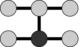
Figure 1: Example of a stencil representation of a PdE. This particular stencil is know as the Crank-Nicolson stencil and is often used to simulate the heat equation (second order in space and first order in time). The discretization variable for space and time are respectively denoted by (k_{2}) and (k_{1}). The gray and black dots represent six data points in two dimensions. The black lines connecting the data represent a linear relation between the data points. In numerical simulations, the black point is calculated as a linear combination of the gray points.
Recursive Hankel matrix
At the basis of the order estimation algorithm proposed in this post lies the concept of the recursive Hankel matrix (\(H_{r}\)) [9]. The measured input-output data is reshaped to reveal linear relations between adjacent data points. For a scalar time series \(u[k]\) with \(k=0,1,2,\dots\), a Hankel matrix \(H\) is defined as,
\begin{equation} H[i,j] = u[i+j-2], \end{equation}
for \(i,j=1,2,\dots\) and \(i\leq n_{1}\) and \(j\leq n_{2}\), with \(H \in \real^{n_{1}\times n_{2}}\). The values of \(n_{1}\) and \(n_{2}\) are user defined parameters for the hankelization and must be chosen “large enough” [10]. When the data depends on several dimensions this definition has to be extended to account for the additional dimensions, resulting in the so-called recursive Hankel matrix.
Recursive Hankel matrix (2D) For a two dimensional dataset \(y[k_{1},k_{2}]\), the recursive Hankel matrix \((H_{r})\) is defined in two steps. First the matrix \(Y_{0|m_{1}-1,j}\) is defined as,
\begin{equation} Y_{0|m_{1}-1,j}= \begin{bmatrix} y_{0,j} & y_{1,j} & \dots & y_{p-1,j} \\ y_{1,j} & y_{2,j} & \dots & y_{p,j} \\ \vdots &\vdots & \ddots & \vdots \\ y_{m_{1}-2,j} & y_{m_{1}-1,j} & \dots & y_{m_{1}+p-3,j} \\ y_{m_{1}-1,j} & y_{m_{1},j} & \dots & y_{m_{1}+p-2,j} \\ \end{bmatrix}. \end{equation}
The parameter \(p\) is a user defined value and must be “large enough”. This is a Hankel matrix where the second coordinate in the data has been kept constant and a Hankelization is carried out over the first coordinate. In the above definition the notation \(y_{k,l} = y[k,l]\) was used. The matrix \(Y_{0|m_{1}-1,j}\) has dimensions \(m_{1} \times p\). The recursive Hankel matrix \(Y_{0|m_{1}-1,0|m_{2}-1}\) is a block Hankel matrix given by,
\begin{equation} \label{eqn:rh} \begin{bmatrix} Y_{0|m_{1}-1,0} & Y_{0|m_{1}-1,1} & \dots & Y_{0|m_{1}-1,q-1} \\ Y_{0|m_{1}-1,1} & Y_{0|m_{1}-1,2} & \dots & Y_{0|m_{1}-1,q} \\ \vdots &\vdots &\ddots & \vdots \\ Y_{0|m_{1}-1,m_{2}-2} & Y_{0|m_{1}-1,m_{2}-3} & \dots & Y_{0|m_{1}-1,m_{2}+q-3} \\ Y_{0|m_{1}-1,m_{2}-1} & Y_{0|m_{1}-1,m_{2}} & \dots & Y_{0|m_{1}-1,m_{2}+q-2} \\ \end{bmatrix} \end{equation}
The parameter \(q\) is a user defined value and must be “large enough”. The size of this matrix is equal to,
\begin{equation*} (m_{1}m_{2})\times (pq). \end{equation*}
The order of this Hankelization is defined as the tuple, \((m_{1},m_{2})\). For a dataset \(y[k_{1},k_{2}]\) of size \(M_{1} \times M_{2}\) and using all the available data for the Hankelization the size of \(H_{r}\) is,
\begin{equation} (m_{1}m_{2}) \times ((M_{1}-m_{1}+1)(M_{2}-m_{2}+1)). \end{equation}
This result is obtained by setting \(m_{1}+p-2 =M_{1}-1\) and \(m_{2}+q-2 =M_{2}-1\). This definition can be extended to a nD dataset by Hankelizing the different dimensions separately.
Gaphical interpretation of the Hankelization process
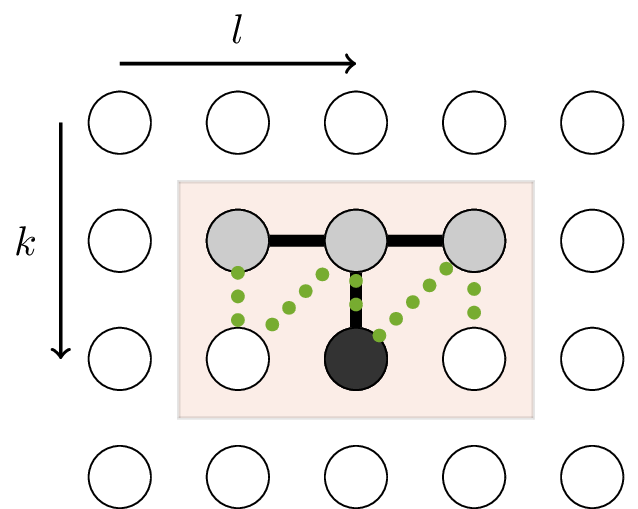
Figure 2: Illustration of the Hankelization method. Inside a predetermined data window, shown here by the box, the data is Hankelized following the dotted line. Each column of the recursive Hankel matrix contains the vectorized data from such a Hankelization window. Also present in the picture is a stencil. The stencil is completely enclosed by the Hankelization window, such that the linear relation of the stencil is captured by the Hankelization window.
The generation of \(H_{r}\) can be illustrated in a graphical way, in which a 2D window slides over the two-dimensional dataset, as shown in Fig 2. The size of the window is equal to \(m_{1}\times m_{2}\). The dotted line in the image illustrates the order of the elements in the columns of \(H_{r}\) with respect to the position in the data matrix. The linear relation associated with this particular stencil is,
\begin{equation} \label{eqn:diff_eqn1} y[k_{1}+1,k_{2}] = \alpha_1 y[k_{1},k_{2}-1] + \alpha_2 y[k_{1},k_{2}] + \alpha_3 y[k_{1},k_{2}+1] \end{equation}
for some parameters \(\alpha_{i}\). In Figure 3 the vectorized data within the Hankelization window is shown. This illustrates the structure of the row space of \(H_{r}\). The important observation is that the information of the linear relation of the PdE is present in the row space of \(H_{r}\), which will result in the rank deficiency of the Hankel matrix. The linear relation is depicted by the black lines connecting the four linearly related points. The left null space of \(H_{r}\) associated with the Hankelization window depicted in Figure 2 with data that satisfies the difference equation \(\ref{eqn:diff_eqn1}\) is spanned by,
\begin{equation} \begin{bmatrix} \alpha_1 & 0 & \alpha_2 & -1 & \alpha_3 & 0 \end{bmatrix} \end{equation}
Example of Hankelization for a two dimensional dataset
To illustrate the concept of Hankelization, a small example is provided for a two-dimensional \(3 \times 3\) dataset,

A Hankelization window of size \(2 \times 2\) is used, indicated by the green square: this window slides over the dataset. This produces the following recursive Hankel matrix,

Every column contains the vectorized data of a shifted Hankelization window. The values of \(p\) and \(q\) from the definition of \(H_{r}\) are both equal to \(3\). The green color on the Hankel matrix indicates the relation between the data matrix and the Hankel matrix. In the next section the properties of this matrix are further analyzed.
Rank of the recursive Hankel matrix
In previous research the recursive Hankel matrix has been introduced in the context of 2D spectral analysis. The rank of \(H_{r}\) is related to the number of rank-one 2D wave functions that make up the dataset \(\mathcal{Y}\) [4]. In this post the rank of \(H_{r}\) is related to the order \(\ref{eqn:nDsystemDiscrete}\). To ensure that a unique solutions exist, some conditions must be satisfied.

Figure 3: Illustration of the column structure of the (H_{r}) matrix. Notice that the stencil is present in the structure of the Hankel matrix. The first, third, fourth and fifth row are linearly dependent. The linear relation is denoted by the black lines. The dotted line is the vectorized line of Figure 2.
Persistency of excitation
Before the rank proposition for input-output systems is provided, the concept of persistency of excitation must be extended to 2D systems. The condition of persistency of excitation ensures that the solutions is unique. For multidimensional input-output systems the boundary condition and the input must be persistently exciting.
Persistently exciting 2D-signal A two-dimensional signal \(y[k_1,k_2]\) for \(k_1=0,\dots,M_1-1\) and \(k_2 =0,…,M_2-1\) is persistently exciting of order \((m_{1},m_{2})\) when the recursive Hankel matrix \({Y}_{0|m_{1}-1,0|m_{2}-1}\) is full rank. Or stated less, the signal \(y[k_{1},k_{2}]\) is not linearly related within a Hankelization window of size \((m_{1},m_{2})\).
The definition of a persistently exciting boundary condition is as follows,
Persistently exciting boundary condition For a two dimensional problem the boundary conditions are one dimensional signals (time series). A boundary condition is persistently exciting of order \(m_{i}\) when the corresponding Hankel matrix \(H_{0|m_{i}-1}\) is full rank [11]. The set of boundary conditions of a PdE is persistently exciting when the boundary conditions are linearly independent.
These two definitions are important to eliminate the effects of “insufficiently rich” input signals. In the context of partial difference equations the distinction between boundary conditions and initial conditions is often made. In this post the initial condition is also referred to as a boundary condition.
Autonomous 2D systems
Autonomous 2D systems are systems with no inputs, represented by the following difference equation,
\begin{equation} \label{eqn:auto} \sum_{i=0}^{n_{1}} \sum_{j=0}^{n_{2}} \alpha_{i,j}y[k_{1}+i,k_{2}+j] = 0 \end{equation}
where \(\alpha_{i,j}\) are the coefficients of the PdE and \((n_1, n_2)\) the order of the PdE.
Rank of \(H_{r}\) for autonomous systems Consider a two-dimensional dataset coming from the autonomous system described by Equation \(\ref{eqn:auto}\) with persistently exciting boundary conditions. The size of the dataset is equal to \(M_{1}\times M_{2}\). The recursive Hankel matrix of order \((m_{1},m_{2})\) from Equation \(\ref{eqn:rh}\), is rank-deficient when,
\begin{equation} \label{eqn:auto-condition} m_{i} > n_{i}, \hspace{3mm} \text{with} \hspace{3mm} 1\leq i \leq 2, \end{equation}
with \((n_{1},n_{2})\) the order of the autonomous difference equation. Stated in a less formal way, the recursive Hankel matrix is rank-deficient when the Hankelization window captures at least the complete stencil of the difference equation. We further assume that the size of the data matrix is large enough such that \(H_{r}\) is a fat matrix (more columns than rows), that is,
\begin{equation} M_{i} \geq 2m_{i}+1, \hspace{3mm} \text{with} \hspace{3mm} 1\leq i \leq 2. \end{equation}
Under the condition of a persistently exciting boundary condition, and a fat \(H_{r}\), the rank of the recursive Hankel matrix is equal to,
\begin{equation} \label{eqn:rank_RH} (m_{1}-n_{1})(m_{2}-n_{2})-(m_{1}m_{2}). \end{equation}
It follows that the dimension of the left-null space is,
\begin{equation} (m_{1}-n_{1})(m_{2}-n_{2}). \end{equation}
The proof of this proposition is found by inspecting the row space of \(H_{r}\). Every column of \(H_{r}\) is equal to,
\begin{equation} \label{eqn:col} \begin{matrix} [y_{k_1,k_2} & y_{k_1+1,k_2} & \dots & y_{k_1+m_{1},k_2} \\ y_{k_1,k_2+1} & y_{k_1+1,k_2+1} & \dots & y_{k_1+m_{1},k_2+1} \\ &&\dots && \\ y_{k_1,k_2+m_{2}} & y_{k_1+1,k_2+m_{2}} &\dots & y_{k_1+m_{1},k_2+m_{2}}]^{T}, \end{matrix} \end{equation}
for some value \(k_{1}\) and \(k_{2}\). Under the condition of Equation \(\ref{eqn:auto}\) there exists a non-trivial linear relation between the elements of equation \(\ref{eqn:col}\). This relation is given by coefficients of the difference equation,
\begin{equation} \label{eqn:null00} \begin{matrix} [\alpha_{0,0} & \alpha_{1,0} & \alpha_{2,0} & \dots & \alpha_{n_{1},0} & 0 & \dots & 0 \\ \alpha_{0,1} & \alpha_{1,1} & \alpha_{2,1} & \dots & \alpha_{n_{1},1} & 0 & \dots & 0 \\ &&&\dots && \\ \alpha_{0,n_{2}} & \alpha_{1,n_{2}} & \alpha_{2,n_{2}} & \dots & \alpha_{n_{1},n_{2}} & 0 & \dots & 0 ]^{T} \end{matrix} \end{equation}
Under the condition of persistently exciting boundary conditions there are no trivial linear relations in the output data \(y\). The only linear relations are formed by the coefficients of the difference equation. To prove the size of the null space we define the matrix \(N_{[k,l]} \in \real^{m_{1}\times m_{2}}\) as follows,
\begin{equation} \label{eqn:beta} N_{[k_{1},k_{2}]}(i,j) = \begin{cases} \alpha_{i-k_{1}-1,j-k_{2}-1}, & \begin{matrix} 0 \leq i-k_{1}-1 \leq n_{1} \\ 0 \leq j-k_{2}-1 \leq n_{2} \end{matrix} \\ 0, & \mbox{ Otherwise. } \end{cases} \end{equation}
This is a sparse matrix containing a block matrix of size \((n_{1}+1)\times (n_{2}+1)\) starting at position \((k_{1},k_{2})\) and containing the coefficients of the PdE. The matrix can be represented in the following way,

The vector obtained by stacking the columns of this matrix and taking the transpose lies in the left null space of \(H_{r}\), this vector is denoted by,
\begin{equation} \mathcal{N}_{k_{1},k_{2}} = \mbox{vect}(N_{[k_{1},k_{2}]})^{T} \in \real^{1\times (m_{1}m_{2})}. \end{equation}
For \(k_{1}\) and \(k_{2}\) both equal to zero this results in the vector of Equation \(\ref{eqn:null00}\). The total number of basis vectors for the null space that can be constructed in this way is \((m_{1}-n_{1})(m_{2}-n_{2})\). This follows immediately from Equation \(\ref{eqn:beta}\) that the left null space is spanned by,
\begin{equation*} \begin{matrix} [\mathcal{N}_{[0,0]};& \mathcal{N}_{[1,0]}; &\dots ; & \mathcal{N}_{[m_{1}-n_{1}-1,0]}; \\ \mathcal{N}_{[0,1]}; &\mathcal{N}_{[1,1]};&\dots ;& \mathcal{N}_{[m_{1}-n_{1}-1,1]}; \\ \mathcal{N}_{[0,m_{2}-1]};& \mathcal{N}_{[1,m_{2}-1]};&\dots ;&\mathcal{N}_{[m_{1}-n_{1}-1,m_{2}-n_{2}-1]} \end{matrix}, \end{equation*}
where \(";"\) indicates that the vectors are stacked. The size of this matrix is equal to
\begin{equation} (m_{1}-n_{1})(m_{2}-n_{2})\times(m_{1}m_{2}) \end{equation}
This proves the proposition.
Input-output systems
For input-output systems the current output not only depends on neighboring output values but also on neighboring input values. These input values must thus be included in the Hankel structure.
Rank of \(H_{r}\) for input-output systems Consider input-output data coming from system \(\ref{eqn:nDsystemDiscrete}\). The size of both the input and output datasets is equal to \(M_{1}\times M_{2}\). Two recursive Hankel matrices \(U_{0|m_{1}-1,0|m_{2}-1}\) and \(Y_{0|m_{1}-1,0|m_{2}-1}\) of order \((m_{1},m_{2})\) respectively from the input and output data are constructed and the columns are concatenated,
\begin{equation} \label{eqn:input_output_hankel} W_{0|m_{1}-1,0|m_{2}-1} = \begin{bmatrix} U_{0|m_{1}-1,0|m_{2}-1} \\ Y_{0|m_{1}-1,0|m_{2}-1} \end{bmatrix} = \begin{bmatrix} H_{u} \\ H_{y} \end{bmatrix} \end{equation}
This matrix is rank-deficient when,
\begin{equation} \label{eqn:size_of_H} m_{i}> \text{max}(n_{i},o_{i}), \hspace{3mm} \text{with} \hspace{3mm} 1\leq i \leq 2. \end{equation}
Or stated in a less formal way, the recursive Hankel matrix is rank-deficient when the Hankelization window captures at least the complete input- and output stencils of the PdE. Under the condition of a persistently exciting boundary condition and input signal, and a large enough dataset, with,
\begin{equation} M_{i} \geq 2m_{i}+1, \hspace{3mm} \text{with} \hspace{3mm} 1\leq i \leq 2, \end{equation}
the rank of the recursive Hankel matrix is equal to,
\begin{equation} \label{eqn:rank_RH_IO} (m_{1}-n_{1})(m_{2}-n_{2})-2(m_{1}m_{2}) \end{equation}
It follows that the dimension of the left-null space is,
\begin{equation} (m_{1}-n_{1})(m_{2}-n_{2}). \end{equation}
The result is the same as for the autonomous case. This is a consequence of the persistently exciting input signal.
The proof this proposition follows from the proof of the proposition for the rank of autonomous systems. Under the condition of a persistently exciting input signal, \({H}_{u}\) is full rank. When the input-output data satisfies the difference equation \(\ref{eqn:nDsystemDiscrete}\), a non trivial left null space exists. The dimension of the left null space is the same as for the autonomous case, and therefore the rank of the matrix is equal to,
\begin{equation} (m_{1}-n_{1})(m_{2}-n_{2})-2(m_{1}m_{2}). \end{equation}
The dimension of the left-null space is equal to,
\begin{equation} (m_{1}-n_{1})(m_{2}-n_{2}). \end{equation}
The previous two proposition relate the rank of \(H_{r}\) to the order of the system and the order of the Hankelization. Based on these results the order estimation algorithm is derived.
Number of independent points in the data matrix
Equations \(\ref{eqn:rank_RH}\) and \(\ref{eqn:rank_RH_IO}\) states that the rank of \(H_{r}\) equals the number of data points that can be chosen freely and independent inside each Hankelization window. These free points are the boundary conditions and the input signal contained inside the window. Once the boundary and input values are fixed, all the internal points can be calculated as a linear combination of these free points. This concept is illustrated in Figure 4. The original stencil, indicated by the white dots, is the same as that from Figure 2. The gray dots are the boundary conditions and the black points are internal points that are linearly related to the boundary. The size of the stencil is \(2 \times 3\), which is related to a difference equation of order \((1,2)\). The size of the Hankelization window is \(4 \times 5\). Plugging in these values in Equation \(\ref{eqn:rank_RH}\) we find that the rank of this matrix is \(4\times 5- 3\times 2 = 11\). This is exactly equal to the number of linearly independent boundary points of the PdE denoted by the gray dots.
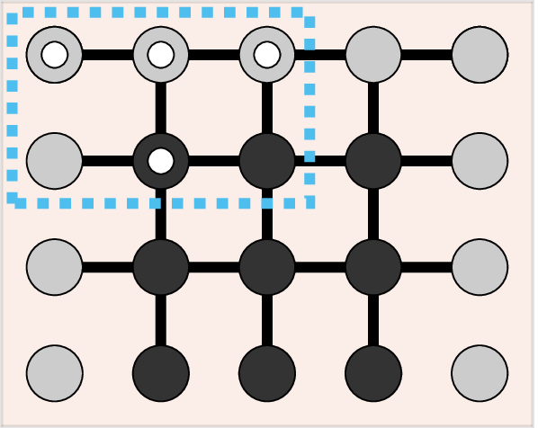
Figure 4: Illustration of the linearly independent points inside the Hankelization window. The stencil used is denoted by the white dots; it is the same as in Figure 2. The dark points are linearly related to the gray boundary points. The size of the stencil is (2times 3) and is shown by the blue dashed box. The rank of the Hankelized data matrix is 11.
Linear relation between rows of Hankel matrices
One thing that has not been shown yet is how the order of the 2D system can be determined based on the rank of \(H_{r}\). To determine the order of the system the dimension of the intersection between two \(H_{r}\) matrices is calculated.
Left, right, top and bottom recursive Hankel matrices
For a two-dimensional dataset, top and bottom is extended to left and right. Graphically the concept of top and bottom is shown in Figure 5. The data matrix is first Hankelized, and afterwards split up in four smaller \(H_{r}\) matrices. In Figure 5 the stencil of a simple PdE of order \((1,1)\) is shown, this PdE is,
\begin{equation} y[k_{1}+1,k_{2}] = y[k_{1},k_{2}+1]. \end{equation}
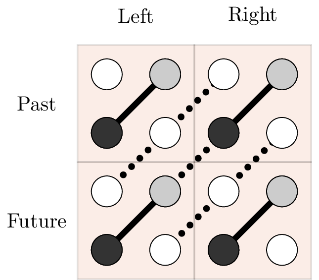
Figure 5: Illustration of the concept of left, right, top and bottom data. In total four matrices are shown, top-left, top-right, bottom-left and bottom-right. The linear combinations between the intersections is shown with dotted lines.
Linear intersection between the row space of \(H_{r}\)
The intersection algorithm for 1D systems was one of the first subspace algorithms to identify input-output state space models [3]. This algorithm splits the Hankel matrix into two separate parts associated with top and future data. The intersection between two matrices contains the top state sequence. Based on this subspace, the size of the state vector and the state sequence are calculated. Consider a 2D dataset coming from an autonomous system. The dataset is Hankelized in four different ways to,
| left | right | |
|---|---|---|
| top | \(Y_{0 \vert m_{1}-1,0 \vert m_{2}-1}\) | \(Y_{0 \vert m_{1}-1,m_2 \vert 2m_{2}-1}\) |
| bottom | \(Y_{m_{1} \vert 2m_{1}-1,0 \vert m_{2}-1}\) | \(Y_{m_{1} \vert 2m_{1}-1,m_2 \vert 2m_{2}-1}\) |
These four matrices contain shifted data with respect to each other, the shift is introduced by changing the starting index of the Hankelization. There is a direct correspondence between these four matrices and Figure 5. The method to determine the order of the PdE calculates the dimension of the intersection between these different Hankel matrices.
Order estimation of two-dimensional difference equations
In this section we show how the order of the PdE is linked to the rank of the \(H_{r}\) matrices. We assume that the conditions of both presented propositions are fulfilled. The derivation is only provided for input-output systems but the results carry over to autonomous systems. The dimension of the left-null space of \(W_{0|m_{1}-1,0|m_{2}-1}\) denoted by \(D\) and is equal to,
\begin{equation} D = (n_{1}-m_{1})(n_{2}-m_{2}). \end{equation}
The next step is to concatenate the left Hankel matrices and the top Hankel matrices, to get,
\begin{equation*} W_{1} = \begin{bmatrix} W_{0|m_{1}-1,0|m_{2}-1} \\ W_{m_{1}|2m_{1}-1,0|m_{2}-1} \end{bmatrix}, \hspace{0mm} W_{2} = \begin{bmatrix} W_{0|m_{1}-1,0|m_{2}-1} \\ W_{0|m_{1}-1,m_2|2m_{2}-1} \end{bmatrix}, \end{equation*}
These two matrices span respectively the same row space as,
\begin{equation} W_{0|2m_{1}-1,0|m_{2}-1} \hspace{10mm} W_{0|m_{1}-1,0|2m_{2}-1}. \end{equation}
The dimension of the left-null space of \(W_{1}\) and \(W_{2}\) is thus respectively given by,
\begin{equation} D_{1} = (2m_{1}-n_{1})(m_{2}-n_{2}), \hspace{3mm} D_{2} = (2m_{2}-n_{2})(m_{1}-n_{1}). \end{equation}
Dividing both \(D_{1}\) and \(D_{2}\) by \(D\) and rewriting the equations it is clear that the order of the PdE is given by,
\begin{equation} n_{i} = \frac{m_{i}(D_{i}-2D)}{D_{i}-D}, \hspace{3mm} \text{for} \hspace{3mm} 1\leq i \leq 2. \end{equation}
The right terms in this expression can be determined numerically by calculating the SVD of the different \(H_{r}\) matrices.
Example: Transport-diffusion
| Window size \(= (m_{1},m_{2})\) | (2,3) | (3,3) | (2,4) | (4,4) |
|---|---|---|---|---|
| \(D\) | 1 | 2 | 2 | 6 |
| \(D_1\) | 3 | 5 | 6 | 14 |
| \(D_2\) | 4 | 8 | 6 | 18 |
| Estimated order \(= n_{1}\) | 1 | 1 | 1 | 1 |
| Estimated order \(= n_{2}\) | 2 | 2 | 2 | 2 |
To illustrate the theoretical results provided in this post a numerical example is presented. In this example we work with data is simulated by,
\begin{multline} \label{eqn:transport-diff_io} y[k_{1}+1,k_{2}] = \rho \left( y[k_{1},k_{2}+1]-2y[k_{1},k_{2}] + y[k_{1},k_{2}-1] \right) \\ + C\left( y[k_{1},k_{2}+1]- y[k_{1},k_{2}-1] \right) + y[k_{1},k_{2}] -u[k_{1},k_{2}], \end{multline}
where \(y\) and \(u\) are respectively the output and input. The index \(k_{1}\) is associated with time and the index \(k_{2}\) is associated with space. The parameters of the PdE are: \(\rho=0.005\) and \(C=0.4\). This equation is the discretized transport-diffusion equation using a forward Euler technique. The input signal is a discrete binary (between 0 and 1) switching signal. Approximately 10% of the data points are randomly chosen to be equal to 1. The boundary conditions are random normal distributed signals. There are two boundary conditions in space and one in time (initial condition). For these random signals the persistency condition is fulfilled. The PdE is second order in space and first order in time. This means that the Hankelization window of size \(2\times3\) is already rank deficient. The results of the order estimation are shown in the table. For every order of the Hankelization that we tried the order of the PdE was estimated correctly. The null space of \(H_{r}\) of order \((2,3)\) is spanned by the coefficients of the PdE. Note that the retrieved order is the order of the PdE and not of the original PDE, in this particular case both orders are the same.
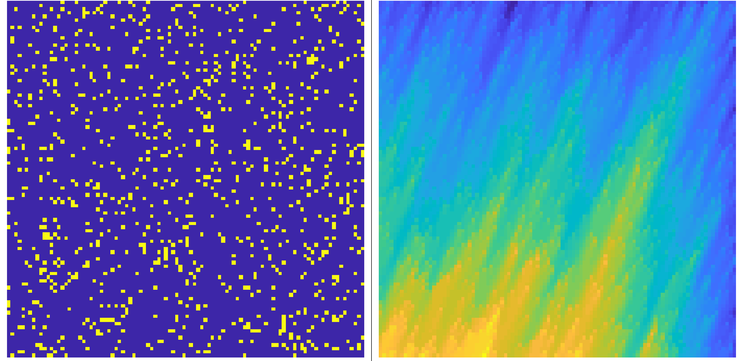
Figure 6: Input-output data for the one-dimensional transport diffusion equation (eqref{eqn:transport-diff_io}). The yellow points represent a high concentration
Conclusion
In this post a method for estimating the order of a partial difference equation has been presented. The method is based on the ideas of the intersection algorithm for 1D systems. First a Hankelization method was presented which can naturally be linked with a window that slides over the data. Next we extended the concept of past and future data from 1D to 2D systems, and introduced the concept of left, right, top and bottom data, resulting in 4 recursive Hankel matrices. From the intersection between the different Hankel matrices the order of the PdE can be calculated. At the moment no subspace method that explicitly uses the matrix intersections has been derived. This post summarized the first results of calculating intersections between Hankel matrices for 2D systems. There are still a lot of research challenges ahead. For example, is there a state sequence between two Hankel matrices like in the 1D case, if so, what is the corresponding state space model? How can these results be linked to the Grasmann dimensionality theorem? All results presented in this post can be extended to PdEs in \(n-\) dimensions.